


Introduction
This project was set up by Data and Computer Science department, Sun Yat-sen University, and Sun Yat-sen Memorial Hospital. It aims to build a framework that could train a model to “learn” to detect any types of cells they want. And the first type they chose is the Eosinophils(EOS) , which is vital in clinical testing and somewhat easy to be recognized.
Two other medical students and I were invited to try the water. The model was supposed to be used in personal computers, especially laptops. We started with three labeled slides. On each of the slides, there are about 100 - 200 Eosinophils. The figure below is an example.

Main Problems
How to train a model that can detect Eosinophils in a “reasonable correctness“ (academic study sometimes starts with an ambiguous aim)?
How to make this model run on laptops?
How to used limited resources for labeling to generate the most labels?
Solutions I applied

First, I tried to use Google’s object detection API in Tensorflow to train a model, which is based on faster-RCNN architecture. It failed, of course, simply because the number of images is too small. Also, I realized the model of faster-RCNN being one hundred more MB, which is quite large, and it is not possible to run on ordinary laptops fast.
Luckily, Kaggle has hosted a competition about cell detections at that moment. From that competition, I met a model architecture, U-net. Many teams in that competition successfully used this architecture. Moreover, it’s fast and relatively small, which fitted our users’ needs. Still, three slides were not enough.
So the first thing was to get enough data. We decided to train a simple CNN model to help us label slides. First, we used watershed and other algorithms to segment cell-like “tiles” from the slides. Then, we used these small images to train a classification CNN model. The model worked well. And we used it to classify the cell-like objects segmented by a watershed algorithm on unlabeled slides. It’s an indirect way to label slides. After that, we just corrected the wrong label, and we could get labeled slides super quickly because the CNN model has labeled many cells. The result like the below. The boxed are the model’s labels, and we used green points to “correct” its labels.

After 40 to 50 slides, we began to use U-net as the architecture for our next model. However, U-net can only generate a possibility hot-map and needs hot-maps to train. Remember what the users asked is the count of cells, not a possibility hot map. So the U-net model cannot work alone, and we had to design a pipeline to have other components complementing the U-net model.
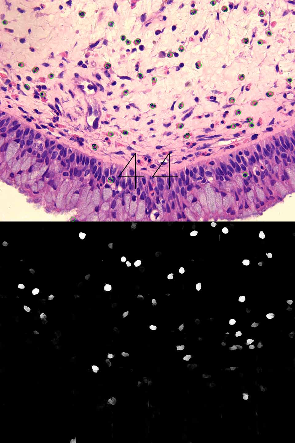
For training, first, we cropped each large slide into small images. Then, we used watershed algorithms to “transform” our previous label as “masks” so that U-net can be trained. When it comes to prediction, we cropped the slide for prediction into small images first; next, we used U-net to generate masks; then, masks were combined into a large mask to match the original slide. Finally, we use watershed and other algorithms to detect the region of cells. Because U-net’s prediction masks will show the interest of regions as white and the background as black, it’s easy for the watershed to separate the cells from this pure background. The final output and its Mask are shown below. Then, we had done it!
For more details, look at in Here.
Results
We randomly sampled 20 well point-labelled images into a test set. By using a different number of training images, we computer how precision, sensitivity and f1_score change as the training image number changes. The “overlap criterion” is defined as an intersection-over-union greater than 0.5.
| true_positive | false_positive | false_negative | precision | sensitivity | f1_score | training image number | |
|---|---|---|---|---|---|---|---|
| 0 | 1089 | 837 | 349 | 0.565421 | 0.757302 | 0.647444 | 10 |
| 1 | 1116 | 462 | 322 | 0.707224 | 0.776078 | 0.740053 | 15 |
| 2 | 1044 | 349 | 394 | 0.749462 | 0.726008 | 0.737549 | 20 |
| 3 | 1115 | 600 | 323 | 0.650146 | 0.775382 | 0.707263 | 25 |
| 4 | 1079 | 327 | 359 | 0.767425 | 0.750348 | 0.75879 | 30 |
| 5 | 1157 | 491 | 281 | 0.702063 | 0.80459 | 0.749838 | 35 |
| 6 | 1113 | 357 | 325 | 0.757143 | 0.773992 | 0.765475 | 40 |
| 7 | 1072 | 343 | 366 | 0.757597 | 0.74548 | 0.75149 | 45 |
| 8 | 1138 | 429 | 300 | 0.726228 | 0.791377 | 0.757404 | 50 |
| 9 | 969 | 236 | 469 | 0.804149 | 0.673853 | 0.733258 | 55 |
| 10 | 1134 | 380 | 304 | 0.749009 | 0.788595 | 0.768293 | 60 |
| 11 | 1101 | 326 | 337 | 0.771549 | 0.765647 | 0.768586 | 65 |
| 12 | 1012 | 255 | 426 | 0.798737 | 0.703755 | 0.748244 | 70 |
| 13 | 1049 | 295 | 389 | 0.780506 | 0.729485 | 0.754134 | 75 |
| 14 | 1036 | 242 | 402 | 0.810642 | 0.720445 | 0.762887 | 78 |

Better Solutions I know now
Check out this article that I published on Medium.
